Implementing the Current Expected Credit Loss (CECL) Model [White Paper]
Table of Contents
Skip to table of contents- Introduction
- What is CECL?
- What can the financial institutions industry learn from other industries?
- How should a financial institution accumulate the data?
- How should a financial institution model expected credit performance?
- How large must a pool be in order to be statistically valid?
- How do I incorporate my financial institution’s performance?
- How does a financial institution incorporate current economic conditions – which is required by the standard?
- How does a financial institution include forecasted changes in macroeconomic conditions – again required by the standard?
- Can I use the CECL information to better manage my financial institution?
- How can Wilary Winn help me with CECL?
- Endnotes
Key Takeaway
Wilary Winn offers comprehensive CECL calculations as well as capital stress testing, concentration risk analyses, and estimates of real return.
How Can We Help You?
Founded in 2003, Wilary Winn LLC and its sister company, Wilary Winn Risk Management LLC, provide independent, objective, fee-based advice to over 600 financial institutions located across the country. We provide services for CECL, ALM, Mergers & Acquisitions, Valuation of Loan Servicing and more.
Released November 2016
Introduction
CECL represents a major change in the way financial institutions estimate credit losses. It requires an institution to estimate life-of-loan credit losses at the inception of the loan. The calculation can be made in a variety of ways, including discounted cash flow, loss rates, roll-rates, and probability of default analyses.
We believe the best analysis technique depends on the type of loan. For example, a financial institution could individually analyze its largest CRE loans based on its knowledge of the borrower and current forecasted economic conditions.
Wilary Winn believes the sheer volume of residential real estate and consumer loans in a portfolio preclude loan-by-loan analyses and are best analyzed using statistical techniques. We use robust discounted cash flow models to produce loss estimates for these types of loans.
ASU 2016-13 Measurement of Credit Losses on Financial Instruments was issued on June 16, 2016. The ASC creates ASC 326. Subtopic 326-20 applies to financial assets measured amortized cost – the CECL methodology. The new accounting is effective in 2020 for financial institutions that are SEC filers. It is effective in 2021 for all others. Early adoption is permitted in 2019.
What is CECL?
CECL is the acronym for the Current Expected Credit Loss Model. In essence, it requires companies to record estimated life time credit losses for debt instruments, leases, and loan commitments. The big change here is that the probability threshold used to determine the allowance for loan and lease losses is removed and FASB expects lifetime losses to be recorded on day one. While CECL affects all companies and financial instruments carried at amortized cost, this white paper focuses on residential real estate and consumer loans because Wilary Winn works solely with financial institutions and we believe these types of loans are best modeled using statistical approaches.
CECL requires a financial institution to recognize an allowance for expected credit losses. Expected credit losses are a current estimate of all contractual cash flows not expected to be collected. That seemingly simple statement begs further explanation. Let’s begin with the contractual cash flows – the amount of principal and interest a financial institution would receive if the borrower made every payment required under the loan agreement. FASB indicates that contractual cash flows should be adjusted for expected prepayments in addition to the expected losses. It further notes that contractual cash flows should not be adjusted for extensions, renewals, or modifications unless a TDR is reasonably expected.
CECL represents a significant change in the way financial institutions currently estimate credit losses. The standard allows financial institution to calculate the allowance in a variety of ways including discounted cash flow, loss rates, roll-rates, and probability of default analyses. Whatever methodology is used, the standard requires that the loss estimate be based on current and forecasted economic conditions. When using a discounted flow technique, the discount rate to be used is the loan’s effective interest rate – the note rate adjusted for discounts and premiums.
What can the financial institutions industry learn from other industries?
While CECL represents a significant change in the way financial institutions currently estimate credit losses, the underlying financial techniques have been used for decades in other industries. We believe the best analysis technique to be used depends on the type of loan. For example, a financial institution could analyze its commercial real estate loans by re-underwriting its largest loans based on its knowledge of the borrower and current and forecasted economic conditions. It could combine this with a historical migration analysis – how many of risk rating ones migrated to lower ratings over time. The focus of this white paper is on residential real estate and consumer loans where the sheer number of loans a financial institution holds precludes a detailed loan-by-loan analysis. Wilary Winn believes that unlike the relatively heterogeneous commercial real estate loans, the relatively homogenous residential real estate and consumer loans can be analyzed using statistical techniques and that financial institutions can benefit from techniques used in other industries. We commence with the asset-backed securities marketplace. Examples would include Collateralized Mortgage Obligations issued by Fannie Mae and Freddie Mac, or securities issued by one of the large auto finance companies.
The issuer of an asset-backed security forms a pool of loans, estimates the cash flow that will arise from the pool and sells securities that have differing rights to the cash flow. For example, an issuer groups a $100 million pool of prime credit auto loans. It then sells three securities: a $65 million senior bond, a $25 million mezzanine bond and a $10 million junior bond. The cash flows arising from the pool of auto loans are allocated first to the senior bond, next to the mezzanine bond, and finally to the junior bond as available. In this way, the senior bond enjoys the most protection from credit losses and receives the lowest yield, while the converse is true for the junior bond.
The fair value of an asset-backed security is equal to the present value of the cash flow expected to be received adjusted for prepayments and expected losses. To derive expected cash flows, a valuation firm will adjust the contractual cash flows for:
- Voluntary prepayments which is called the conditional repayment rate – (“CRR”)
- Involuntary prepayments or defaults, which is called the conditional default rate – (“CDR”)
- Loss severity or loss given default – which is the loss that will be incurred (“loss severity”)
We note that CRR plus CDR is equal to the overall prepayment rate – the so called conditional prepayment rate or “CPR”.
The valuation technique can be easily adapted to meet the CECL requirements – the only difference is the discount rate used. In the case of determining fair value, the interest rate used is equal to the market rate an investor would require, whereas in the case of CECL it is the effective rate of interest on the loan. A second major advantage to the use of this technique is that it relies on the use of the same credit indicators financial institutions now use to underwrite loans and manage their loan portfolios, including FICO, loan term, and loan-to-value percentage.
The exposure draft allows for the use of other methods, including loss rates, roll-rates, and probability of default methods, which “implicitly” include the time value of money.
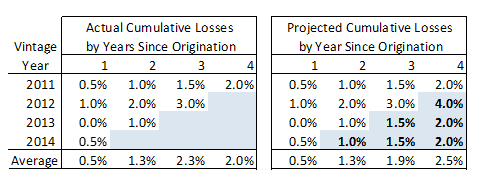
The insurance industry has long been required to forecast expected life time losses, and their work can also provide insights into CECL. One way insurers have estimated losses is through analysis of loss rates by year of origination. In this case, an insurer compares the loss rate incurred for one vintage year to the loss rate per another vintage year to estimate life-time losses. Following is a highly simplified example. Let’s say we have a group of auto insurance policies with a four-year life.
Policy year 2011 experienced the following loss rates:
- 0.5% for 2012 – year 1
- 1.0% for 2013 – year 2
- 1.5% for 2014 – year 3
- 2.0% for 2015 – year 4
Policy year 2012 is performing worse and has the following loss rates:
- 1.0% for 2013 – year 1
- 2.0% for 2014 – year 2
- 3.0% for 2015 – year 3
Because the loss run rate for policy year 2012 is twice that of 2011, the estimated losses for policy year 2012 in 2016 would be 4% – two times the year 4 run rate of the 2011 pool. See the table shown below.
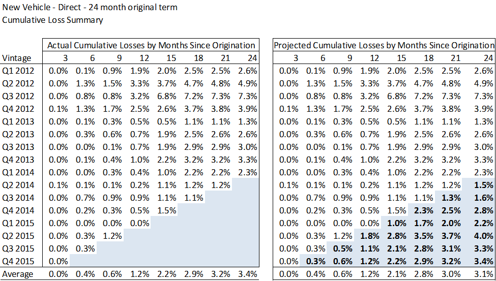
A more complex example of a vintage analysis on 24 month term auto loans is shown below.
A strong caution when using roll rate analyses is that the standard requires a financial institution to adjust for current conditions and for reasonable and supportable forecasts. These requirements can be difficult to apply when using this modeling technique. For example, if a financial institution at the end of 2008 believed housing prices would drop precipitously in 2009 and 2010, then by how much would it upwardly adjust its roll rate analysis? A second difficulty with roll rate analyses is that voluntary prepayments can have a dramatic effect on the remaining balance making it more difficult to compare one year’s results to another. Wilary Winn believes the economic adjustment requirements and the effect of prepayments are much more easily satisfied using a discounted cash flow analysis as described in detail later in this white paper. Another advantage of using discounted cash flow techniques is that the resulting cash flows can be used to estimate fair value, whereas this is not the case for roll rate analyses.
How should a financial institution accumulate the data?
First, we believe that a financial institution should group loans based on similar characteristics and based on its knowledge of the factors that most strongly affect credit performance. For example, we believe a financial institution should analyze first lien residential mortgage loans separately from second lien mortgages and that the first lien group be further subdivided between fixed and variable rate mortgages. As another example, we believe that auto loans should be divided into four major categories because new versus used car loans perform differently, as do loans originated by the financial institution versus those obtained through a dealer:
- New direct
- New indirect
- Used direct
- Used indirect
We note that the formation of the loan groupings can be strongly informed by a thorough concentration analysis. As we indicate further on in the white paper, these are only the major groupings for data accumulation and the expected future performance of the loans should be based on even finer strata. In fact, we model residential real estate loans at the loan level.
Wilary Winn believes financial institutions should go back in time at least 10 years in order to include results prior to and in the midst of the financial downturn. The information should include macroeconomic indicators, both at the national level and within the financial institution’s geographic footprint including:
- Unemployment rate
- Real median income
- Changes in GDP
- Change in housing prices
- Change in used auto prices
It should also track interest rates both short- and long-term.
A financial institution should also accumulate specific information regarding the performance of the loan portfolio including:
- Delinquency rates by loan grouping by quarter
- Balance of the defaulted loan and the date of the default
- Proceeds from liquidation of the defaulted loan
- FICO and combined LTV of the loan at the time of default
- Balance of a prepaid loan and date of the prepayment
The approach a financial institution plans to use to calculate lifetime losses thus affects the way it accumulates the data. If a financial institution plans to use a discounted cash flow analysis it should accumulate the information by the loan groups it has identified. We encourage financial institutions to ensure they thoroughly “scrub their data” to avoid the risk of being whipsawed on CECL estimates due to changes in loan attributes or credit indicators.
If the financial institution plans to use a roll rate methodology then it should further divide its loan groupings by year of origination.
We recognize that other experts are recommending that financial institution’s go back only as far as the expected life of the loan. For example, perform a 3 year look back for an auto loan with an expected 3 year life. Wilary Winn strongly counsels against this shortcut because the financial conditions an organization is currently facing or expecting to face could be quite different than the most recent few time periods. To accurately predict loan performance, a financial institution must understand how its loans will perform in “good times and bad”. It thus must have data that includes a significant downturn in the economy. We believe that the more information a financial institution has, the more defensible its position to its regulators and external auditors. We believe the more precise the model, the less pressure a financial institution will have to cushion its allowance for potential modeling error.
How should a financial institution model expected credit performance?
Wilary Winn believes a financial institution should begin its credit analysis with the factors it believes are predictive and divide the portfolio accordingly. As we indicated earlier, residential real estate loans should be divided between first lien and second lien and further divided between fixed rate and variable rate. HELOC’s should be modeled separately from closed-end seconds. Loans with balloons should be modeled separately from those with full amortization. Similarly, auto loans should be divided between new and used, and further subdivided by direct versus indirect.
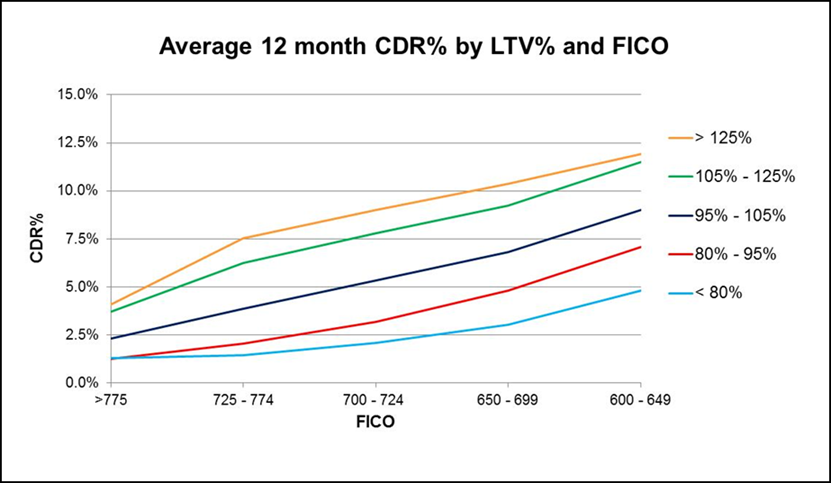
In addition, the modeling should be based on the inputs most highly correlated to expected losses. For example, our research has shown that the performance of residential real estate loans is highly correlated to FICO and combined LTV. Neither factor alone is nearly as predictive as the two combined. This makes intuitive sense. For example, a first lien residential real estate loan with a FICO of 720 and an LTV of 80% would have a very small chance of default. On the other hand, a loan with a FICO of 720 and an LTV of 150% would have a higher chance of default and a higher loss severity. Similarly, a loan with a FICO of 550 and an LTV of 150% would have a high chance of default and a high loss severity whereas a loan with a FICO of 550 and an LTV of 50% would have a much lower chance of default. Moreover, if it defaulted would have a smaller percentage loss or perhaps no loss at all. The graph below shows how defaults increased post-recession as FICOs decreased and LTVs increased and confirms these relationships.
An example of a CECL calculation for a portfolio of residential real estate loans is attached as Appendix A. Wilary Winn notes that we run the analysis at the loan level and aggregate the FICO and LTV bands for ease of presentation only.
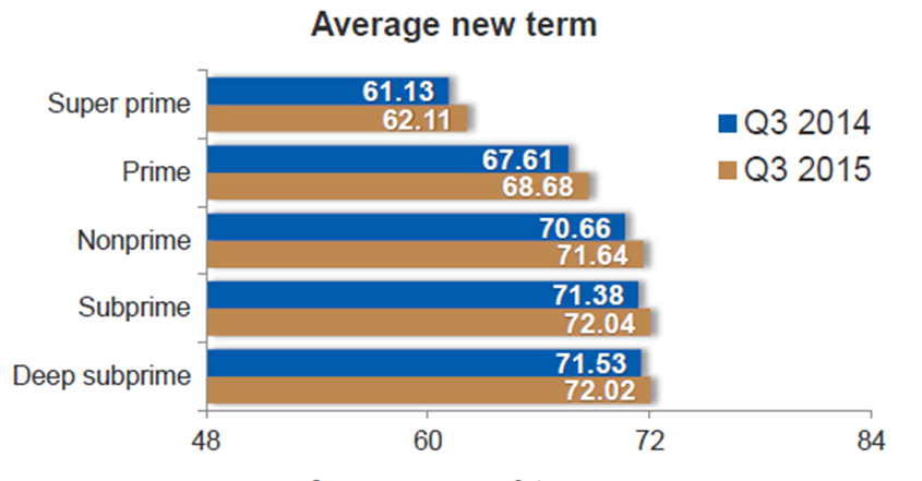
As another example, our research has shown that FICO and loan term are predictive of the credit performance of auto loans. A loan with a FICO of 660 and a term of 84 months will likely perform worse than a loan with a term of 48 months. Again, this makes intuitive sense, if a borrower is stretching to buy a car by accepting a longer term in return for a lower monthly payment, their chance of defaulting is ultimately higher. Moreover, the longer loan term heightens the risk of required expensive repairs to both used and new cars. In addition, the longer loan term will generally exceed the drivetrain warranty for a new car. The chart below shows the industry average term at origination by credit worthiness of borrower.
The task of identifying predictive credit factors can seem daunting. Wilary Winn believes that financial institutions can benefit from the work performed by other industries. For example, we have found research performed by the major ratings agencies to be quite informative. The rating agencies have white papers that detail their approach to rating various types of asset-backed securities including auto loans, commercial and industrial loans, and residential real estate loans. The credit reporting agencies also offer insights into expected credit performance including quarterly updates. The advantage that these national organizations have is that they can base their research on extremely large loan pools.
Using these types of studies as a starting point, we believe the best way to identify predictive credit factors is to run regression analyses in order to determine correlation rates. Informed by the research performed by others, Wilary Winn has spent years accumulating loan performance information. We have run regression analyses and back-tested predicted performance to actual performance.
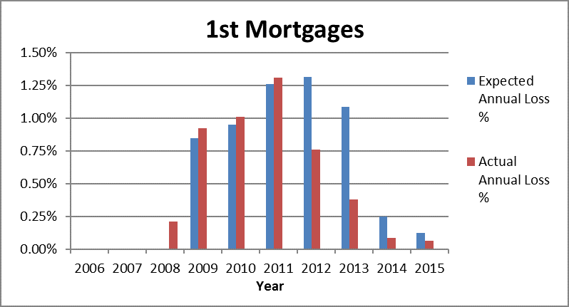
As an example, when we first started performing our annual analyses of loan portfolios as of December 31, 2008, we projected the average annual loss on first mortgages to be 0.85%. At the time, many of our clients viewed our estimate as too conservative given that their loss rates in recent previous years averaged well under this rate. Our clients experienced actual losses of 0.92% in 2009. As shown in the graph, our predictions for the following two years were nearly identical to the actual results our clients experienced and far in excess of their annual loss rates prior to 2009. We note that for 2012, we predicted a loss rate of 1.31% while our clients’ actual losses were 0.76%. Similarly, we forecast a loss rate of 1.09% in 2013 and the actual loss rate was 0.38%. Our estimate for 2012 was too high because we did not incorporate the dramatic forecasted increases in home prices into our model in an effort to avoid whipsawing our results if the increases did not come to fruition. We also capped our housing price appreciation assumption for 2013 which contributed to forecast again coming in too high. Based on our back testing, we also recognized that we needed to improve our models in order to better account for the rapid changes in housing prices. We thus adjusted our models to vector our base default rate monthly for the life of the loan based on housing price appreciation and loan amortization. This improvement in our modeling brought our forecasted results much closer to the actuals in 2014 and 2015.
This begs two questions for an individual financial institution that plans to do its own research:
- How many units have to be in the loan pool in order to be considered statistically valid?
- If after dividing my loans into predictive categories, I am left with too few loans to be statistically significant, then how do I adjust the industry wide inputs to reflect my institution’s specific performance?
How large must a pool be in order to be statistically valid?
To help us answer the first question, we turned to Professor Edward W. Frees, the Hickman Larson Chair of Actuarial Science at the University of Wisconsin – Madison. (For the sake of relative simplicity, we will focus on loan defaults only and omit loss given default or loss severity.) The risk of a loan defaulting is binary – it either does or does not default. In order to determine a required sample size a financial institution needs to determine the margin of error that it can tolerate and the amount of confidence it must have in the results. For illustrative purposes, let us assume we can tolerate a sampling error of 3% with a 95% confidence level.
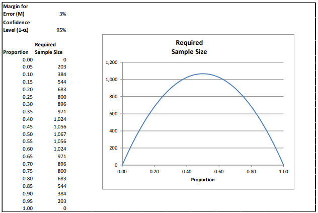
As the reader can see, the required sample sizes are relatively small when the probability of default nears highly certain or highly uncertain (1 or 0, respectively).
We can build on this idea by considering binary risks that are grouped into categories. In this next example, we divide loans into FICO buckets assigning default probabilities from our previous industrywide research – loans with FICOs of 780 and above have a .03% chance of default while loans with FICOs below 500 have a 23.06% chance of default.
In statistical parlance, these differing probabilities of default are called proportions. Because we have differing proportions, we will vary our margins of error in order to derive realistic required sample sizes.
To help us determine the margins of error by FICO band, we turn the idea of financial statement materiality. Let us say we have a financial institution with a $500 million of total assets. For the sake of simplicity, we will assume it has $200 million of fixed rate mortgages and an allowance for loan losses of 0.25% or $500,000. Using a fifteen percent materiality threshold for the allowance we need to produce a loan loss estimate that is reliable to plus or minus $75,000. Let us assume an average loss severity of 23 percent – the rate for FNMA and FHLMC prior to recent financial downturn. We can then set our margin of error tolerances based on the dollar amount of loans in each FICO bucket, the number of probable defaults, and the average loss severity.
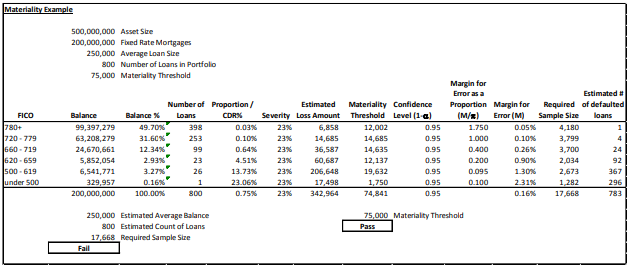
In this case, we can see that the financial institution has an insufficient number of loans in its portfolio to be able to derive a statistically valid result. The required sample size is 17,668 loans in order for our expected credit loss estimate for the portfolio to be within $75,000 and the financial institution has just 800 loans. As a result, it will need to rely on information derived from larger pools. We can also see that our example financial institution does not have sufficient information in the lower risk FICO groupings – the areas with the greatest potential risk. For example, to be statistically accurate a financial institution would need 3,700 loans in the 660-719 group for which we would expect 24 defaults. Our sample financial institution has just 99 loans in this cohort. We believe that this data shortfall for lower quality loans will continue as we continue to move forward into the future from the financial downturn. Nevertheless, we want to incorporate the financial institution’s actual performance into our loss estimates.
Before we show how that can be done, we note that this table is highly simplified and that a minimum we would want to have historical performance data based on FICO and combined LTV, similar to Appendix A. This reinforces the need for larger data pools because slicing the groupings again obviously results in fewer loans per predictive indicator.
How do I incorporate my financial institution’s performance?
To help us with the second question of incorporating a financial institution’s actual results, we again turned to Professor Frees and we can again learn from another industry. The insurance industry addresses the issue with a concept called “credibility theory”. The idea is to blend a financial institution’s loss rates with industry-wide loss experience. There are many varieties of credibility theory that can be used depending on company expertise and data availability. One variety is “Bayesian credibility theory” that employs statistical Bayesian concepts in order to utilize a company’s understanding of its business and its own experience.
We will use the 500-619 FICO group for our example. Assuming the average loan size for this cohort is also $250,000, we have 26 loans in the group. To estimate our sample size, we used an industry average default rate of 13.73% for the group and our required sample size was 2,673 loans. We assume that 367 of the 2,673 loans in the group will default. To continue our example, let us assume that the financial institution’s actual recent default experience was 49.68% for this FICO cohort. While it first appears that the financial institution’s default probability is worse than the industry average, this could also be due to chance variability. To avoid this potential outcome, we want to incorporate the financial institution’s actual performance into our CDR estimate in a statistically valid way. To do this, we want to be 95% confident that our estimate is within 9.5% of the true default probability, consistent with our required sample size inputs.
Credibility estimators take on the form:
New Estimator = Z × Company Estimator + (1 − Z) × Prior (Industry) Estimator
Although there are many variations of this estimator, most experts express the credibility factor in the form:
Z = n/(n+k)
for some quantity k and company sample size n. The idea is that as the company sample size n becomes larger, the credibility factor becomes closer to 1 and so the company estimator becomes an important in determining the final “new estimator.” In contrast, if the company has only a small sample n, then the credibility factor is close to 0 and the external information is the more relevant determinant of the final “new estimator.”
For our example, using some standard statistical assumptions, one can show that:
k = 4/(L^2 * Prior Estimator)
Here, “L” is the proportion desired (9.5% in our example, margin for error as a proportion or M/π in our prior example notation). Our prior estimate for defaults (“CDR” or proportion) for this band was 13.73%.
To continue, this is k= 4/(L^2 * Prior Estimator) = 4/(9.5^2 * 0.1373) = 3,228. With this, we have the credibility factor Z = 26/(26 + 3,228) = 0.80%
Our final CDR estimate for the 500 to 619 FICO band is equal to our company input (49.68% * 0.80%) + (1 – 0.80%) * 13.73% or 14.02%. We have thus incorporated the financial institution’s performance in this loan category into our CDR estimate in a statistically valid way deriving a lower estimate than if had we the institution’s actual results only.
How does a financial institution incorporate current economic conditions – which is required by the standard?
This can be done in many ways. If a financial institution is using static pool analyses, it can compare today’s economic conditions to past time periods when conditions were similar. The largest constraint here is to ensure that underwriting conditions and other factors are similar.
Wilary Winn believes the discounted cash flow estimate offers a better and more reliable alternative. Many financial institutions are already obtaining refreshed FICO scores and updated estimated appraised values (AVMs) as part of their loan portfolio monitoring and managing processes. Wilary Winn believes these updated inputs are very good indicators of current economic conditions and are predictive of future performance.
How does a financial institution include forecasted changes in macroeconomic conditions – again required by the standard?
This can also be done in several different ways. Those using static pools could adjust their loss rates using techniques similar to the environmental and qualitative processes used today. A financial institution is essentially making a top-down adjustment.
Wilary Winn believes the use of a discounted cash flow analysis allows for a bottom-up and therefore more reliable approach. For example, when we are modeling the performance of residential real estate loans, we begin with an updated combined LTV based on a recent AVM. To include short-term changes in housing prices, we utilize forecasts by MSA. Longer term, we incorporate the forecasted change in national housing prices. In this way, we incorporate short-term changes with which we have more certainty with a national forecast that is driven by forecasted economic conditions and historic performance. We use these estimates to change our loss severity estimates. Our models also include a dynamic default vector that is tied to forecasted changes in housing prices. We change our rate of default based on changes to the estimated LTV given normal amortization, curtailments, and changes in housing prices. In this way, we are adjusting our loss estimates based on macroeconomic forecasts.
Another example of a bottom-up approach is the modeling of auto loans. Our research shows that the performance of auto loans is highly correlated with changes in the unemployment rate. We can thus dynamically change our base default vector based on the short-term forecasted unemployment rate in our client’s geographic footprint. We combine this with the forecasted change in the national unemployment rate given less certainty as our estimates go further into the future.
These are two examples of many possibilities a financial institution could utilize depending on what it learns from its correlation research. Because actual and expected changes in macroeconomic conditions must be include in the CECL determination, we encourage financial institutions to carefully consider how they will incorporate these factors in order to avoid whipsaws in loss estimates.
Can I use the CECL information to better manage my financial institution?
Many would argue that these bottom-up approaches, while more predictive, are more work than more simplified vintage analyses to generate estimates for the allowance.
Wilary Winn heartily agrees and believes that that the more robust analyses make sense only when a financial institution plans to use them to better manage its business. For example, we believe that a thorough understanding of credit indicators and conditions can lead to more sophisticated risk-based pricing and greater profitability. We further believe the knowledge gained through these analyses can be used to develop robust stress tests for capital resulting in better and safer capital allocations. We note that if a financial institution plans to incorporate its CECL analyses and into risk-based pricing and capital stress testing, that it consider lowering the error thresholds and increase its sample sizes, thus relying on more industrywide inputs.
How can Wilary Winn help me with CECL?
We can help you ready your institution in several ways.
CECL Estimate
At a minimum, we can estimate the effect that CECL will have on your Allowance for Loan and Lease Losses, based on the FICO and LTV information you have available, using the discounted cash flow and statistical techniques we have described in this paper.
Asset Liability Management
We currently provide our ongoing ALM clients with a CECL compliant estimate of loan losses each time we run their analyses.
Concentration Risk and Capital Stress Testing
Wilary Winn has recently been engaged by several of our clients to combine our life-of-loan credit and prepayment forecasts with concentration risk and capital stress testing analyses. We believe these engagements represent the most powerful use of our analytical models.
Wilary Winn believes that excessive concentrations in type of assets or liabilities can lead to credit, interest rate and liquidity risk. Most concentration risk policies that we have seen address interest rate risk. Wilary Winn believes that while interest rate risk related to concentration is important, we believe credit risk is the most critical because excessive concentrations of credit have been key factors in banking crises and failure. As we analyze loan portfolios, we are not addressing the traditional concentration risk arising from large loans to a few borrowers. We are instead addressing the risk that “pools of individual transactions could perform similarly because of a common characteristic or common sensitivity to economic, financial or business developments1.”
We first perform data mining to identify concentrations in investments, loans, and deposits recognizing that the risk can arise from different areas and can be interrelated. For example, a financial institution could have an indirect auto loan portfolio sourced from a limited number of dealers. Understanding the percentage of the portfolio arising from each dealer and their relative credit performance (FICO and delinquency) would be important in understanding and managing credit risk. As another example, a financial institution could have a geographic concentration of residential real estate loans making it vulnerable to a downturn in real estate prices in a particular area. An example of interrelated risks would be an institution with a concentration of long-term residential real estate loans and a relatively large portfolio of agency mortgage backed securities. It would have credit risk from the loans, and heightened interest rate risk from the combination of the loans and the securities.
Based on the concentrations we identify we perform credit, interest rate and liquidity stress testing in order to help our client refine its existing concentration risk thresholds. The updated concentration thresholds are based in large part on the effect these stress tests have on the financial institution’s level of capital. We believe that an additional benefit of this work relates to risk-based pricing and more efficient use of capital.
Endnotes
- OCC Comptrollers Handbook – Concentrations of Credit ↩︎