CECL Models: Comparing WARM to DCF [White Paper]
Key Takeaway
We provide ALM and CECL solutions that help our clients measure, monitor, and mitigate balance sheet risk on an integrated basis. We consider credit, interest rate, and liquidity risk holistically. We charge a fee for our advice and do not rely on commissions, so we can remain objective. We simply want what is best for our client.
How Can We Help You?
Founded in 2003, Wilary Winn LLC and its sister company, Wilary Winn Risk Management LLC, provide independent, objective, fee-based advice to nearly 600 financial institutions located across the country. We provide services for CECL, ALM, Mergers & Acquisitions, Valuation of Loan Servicing and more.
Released December 2023
Introduction
This white paper focuses on two of the primary models used to estimate CECL reserves – weighted average remaining maturity (“WARM”) and discounted cash flow (“DCF”). We have chosen these two models as fence posts in the continuum of models used for CECL.
The WARM model is relatively simple and is based on a backward look. Because it is retrospective, it is not predictive when macroeconomic conditions change and requires extensive Q & E adjustments in those conditions. Conversely, the DCF model is prospective in nature and is highly predictive.
Using our multi-billion-dollar, multi-year dataset, this white paper shows how a WARM model would have performed in the financial crisis of 2007 through 2009 and the years after. We also show how the Wilary Winn DCF models actually performed over the same time frame.
Important Elements
We begin with the standard. Some of the most important elements within the CECL framework are the:
- Need to include macroeconomic considerations – past events, current conditions, and reasonable and supportable forecasts.
- Requirement to use relevant forward-looking information.
- Requirement that if outside of industrywide data is used, it must be relevant and reliable.
- Life-of-loan calculations and need to consider prepayments.
Credit Losses
Credit losses are comprised of two components – a loan default and the loss incurred on default. The loss on default is based on the loan amount at liquidation and the value of the collateral supporting it. Most models, including WARM, are based on the total loss rate which combines the probability of default with loss to be incurred. The superior predictiveness of the DCF model is due in part to modeling the two separately.
Another very important consideration is that loss rates are not linear. Loans with low credit scores default at far greater rates than those with high credit scores. In practice, this means that the more granular the model, the more predictive it is. Consider this simple example of a portfolio of five residential real estate loans. A loss prediction based on the portfolio average FICO score and loan-to-value ratio results in far too low a loss estimate.
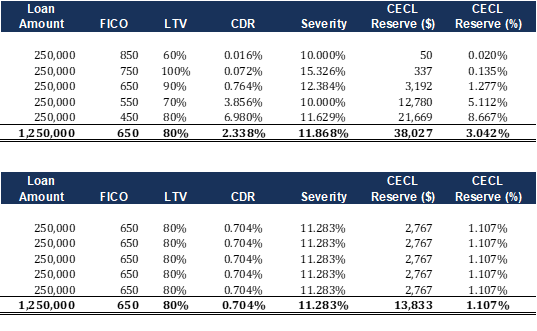
We further note that credit scores migrate over the life of the loan and that collateral values change as well. This is an inherent limitation of aggregate loss rate models such as the WARM method where the effects of these changes must be considered top down. On the other hand, DCF models rely on updated credit scores and collateral values. These key drivers are thus known at the modeling date and their effects need not be inferred.
Weighted Average Remaining Maturity (WARM)
For this model, a financial institution derives a loss estimate for a segment of the loan portfolio based on a lookback period. It then applies this average annual loss rate to its estimated remaining balances based on contractual maturities and estimated prepayments. The annual loss rate is applied to the outstanding remaining balances and the estimated losses are totaled to derive the reserve.
Modeling Considerations
The calculation is:
Portfolio balance x Expected loss rate x Weighted average remaining maturity
Let’s look at each WARM method calculation component in detail.
Portfolio Balance
Most WARM analyses use aggregate call report categories. There are 13 different categories on the call report:
- Unsecured Credit Card Loans
- Payday Alternative Loans
- Non-Federally Guaranteed Student Loans
- All Other Unsecured Loans/Lines of Credit
- New Vehicle Loans
- Used Vehicle Loans
- Leases Receivable
- All Other Secured Non-Real Estate Loans/Lines of Credit
- 1- to 4-Family Residential Property Loans/Lines of Credit Secured by 1st Lien
- 1- to 4-Family Residential Property Loans/Lines of Credit Secured by Junior Lien
- All Other (Non-Commercial) Real Estate Loans/Lines of Credit
- Commercial Loans/Lines of Credit Real Estate Secured
- Commercial Loans/Lines of Credit Not Real Estate Secured
The paucity of portfolio segments makes this model far less predictive than other types of models. For example, all first lien residential real estate loans are included in one broad category. This means that the model does not differentiate by term, credit score, interest type, or purpose. The WARM loss rate thus, for example, combines high FICO, low LTV, fixed rate loans with low FICO, high LTV, adjustable-rate loans. To be predictive, the existing portfolio must have a very similar loan mix, loan attributes and credit indicators to recent and forecasted portfolios, which is unlikely.
Expected Loss Rate
The expected loss rate under the WARM method is based on a lookback – generally three years – of net annual charge-offs. For this variable to be predictive, forecasted macroeconomic conditions must be very similar to the conditions in the lookback periods. This again is unlikely. For example, if the forecasted rate of unemployment is higher than that in the lookback periods, the calculated expected loss is understated.
A second major limitation is that the forecasted loss rate is in aggregate. This assumes that the forecasted incidence of default and the loss incurred on default remain similar to the lookback periods. This further assumes that changes in the value of the collateral in future periods must be similar to the changes in recent prior years. For example, if housing prices are expected to decline in future periods and had increased in the lookback periods, the expected calculated loss is understated.
To compare the models, we are going to look at the credit losses in first lien residential real estate loans originated from 2006 through 2022, incorporating years before and after the severe downturn in housing prices1. Using a three-year lookback, the WARM model shows:
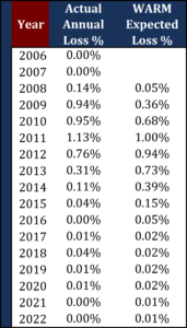
The WARM model understates the loss rates in 2009 through 2011 and then overstates the loss rates in 2012 through 2022. The model thus fails to achieve a main goal of CECL, to bolster reserves in the face of an economic downturn.
Prepayments
The WARM is based on contractual maturity and expected prepayments. Most WARM models use a lookback analysis to estimate prepayments. This can result in decidedly incorrect results. For example, if expected prepayments are modeled too high, the loss is understated. The converse is also true – if modeled expected prepayments are modeled too low, the loss could be overstated.
Voluntary prepayments are largely based on the loan’s interest rate relative to market interest rates. A borrower that has an interest rate higher than the market rate has an incentive to refinance. Let’s use a very simplified example of a three-loan portfolio. Each is a 30-year fixed rate first lien mortgage loan. The first loan has a rate of 3.75%, the second has a rate of 4.25%, and the third has a rate of 7.0% – an average of 5%. Let’s say market interest rates are 4%. The average utilized in the WARM method implies that every borrower in the portfolio has an incentive to refinance, yielding a high prepayment forecast. However, the 3.75% borrower has no incentive and the 4.25% borrower has little incentive. In truth, only one-third of the portfolio is subject to prepayment.
Let’s look at the rate of prepayments in residential real estate loans from 2017 through 2022 – the years where we saw significant changes.
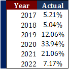
Let’s use 2020 and 2022 as examples. Using a three-year lookback, the WARM model prepayment input for 2020 would be 7.4%, whereas the actual rate was 33.9%. The WARM model severely underestimated prepayments in 2020 because the calculation itself is retrospective – it could not directly incorporate the dramatic fall in interest rates arising from the impact of COVID-related economic stimulus. Similarly, in 2022 the input would be 22.3% compared to the actual of 7.2% because the WARM method lookback calculation included the rapid prepayment rates from 2020 and 2021, when in fact market interest rates had increased significantly from the 2020 floors.
The annual prepayment example is highly simplified. The table below reflects a static pool analysis showing the actual prepayment rates for origination vintages 2016 through 2021. Of particular notice are the rapid prepayments of the 2018 and 2019 vintages in calendar 2020. The table further illustrates the limitations of a WARM analysis.
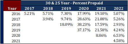
Higher expected prepayments lower the WARM and the resulting credit loss calculation, while lower expected prepayments increase the expected loss.
Model Results
Of course, the “proof is in the pudding,” so let’s look at how the model would have done from 2009 through 2022 by combining expected loss rate and WARM2. The first table is in percentages and the second table shows the dollar effect using a static $500 million loan portfolio. We note that in this case we are modeling a segment of the residential real estate portfolio, making the calculation more accurate than if we ran it at the call report level.
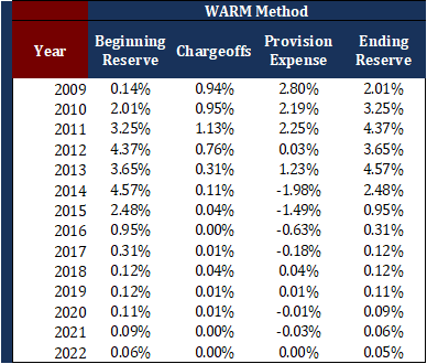
We can see the WARM model causes the financial institution to continue to add to its reserves in 2009, 2010, and 2011. It catches up by 2012. In 2013, the required reserve increases as the average life increases from 3.86 years in 2012 to 6.23 years in 2013. The financial institution then releases reserves in 2014, 2015, and 2016.
The dollar effects are shown below.
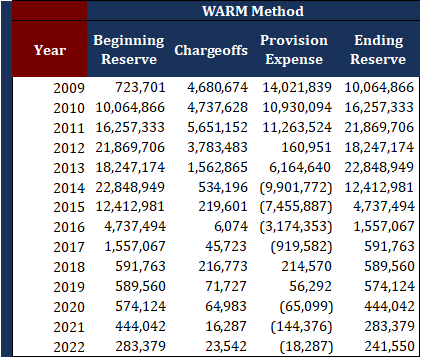
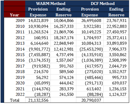
We can see the organization records more than $10 million of expected credit losses each year in 2009, 2010, and 2011 utilizing the WARM method. It then releases nearly $10 million of expected losses in 2014.
Model Transparency
The primary advantages of the WARM model are that it is a straightforward calculation, and the historical loss rate is relatively easily verified.
The simplicity of the model results in a low level of predictiveness, especially under stressed economic conditions, and the need to adjust the calculated results with qualitative and environmental factors.
Other Considerations
To be predictive under the WARM method, the loans need to have similar credit attributes. Changes in underwriting or loan offerings can be very difficult to include. Moreover, the model has a single purpose: to establish a credit reserve. For example, while the outcome can be overlaid into an ALM model, it is not dynamically linked to the ALM modeling results.
In conclusion, the WARM model:
- Relies on simple calculations;
- Is for a single use – estimating the reserve;
- Is retrospective;
- Is slow to correct itself for changes in loan attributes, borrower creditworthiness, and actual and forecasted macroeconomic conditions as the lookback period is three years and recent results would comprise only one-third of the input derivation;
- Is not predictive, and as a result;
- Can require extensive qualitative and environmental adjustments.
Discounted Cash Flow (DCF)
We believe the DCF model has the optimal combination of transparency and predictive power. The model begins with contractual cash flows based on the attributes of the loan at the time of modeling, including loan amount, interest rate and loan term. The total contractual cash flows are then modified to derive expected life-of-loan cash flows. The following variables are used:
- CRR – conditional repayment rate – voluntary prepayment
- CDR – conditional default rate or involuntary prepayment
- Loss severity – loss upon liquidation
The result is that losses are estimated monthly over the life of the loan, after accounting for loan amortization, curtailments, prepayments, and changes in the value of the collateral.
Modeling Considerations
Credit losses are based on the sum of the product of probable defaults (CDR) and the losses incurred on a default (loss severity). Defaults for residential real estate loans are highly correlated to the combination of the borrower’s FICO score and the loan-to-value ratio. We use refreshed FICO scores and updated AVMs at the time of modeling because they directly show the recent and current macroeconomic effects to the borrower’s creditworthiness and the collateral. We need not make an inference; we know the outcome.
The likelihood of default is based on analyzing how loans with similar credit attributes and collateral values fared over the most recent full business cycle, given the current macroeconomic forecasts. Loss severity is based on the value of the underlying collateral relative to the outstanding loan balance at the time of default. The loan level calculation is dynamic, as the outstanding loan balance changes monthly going forward due to amortization and expected prepayments, and the value of the collateral changes based on forecasted changes in housing prices.
Under the DCF method, prepayments are modeled directly based on the loan’s interest at the time of modeling, forecasted changes in market interest rates, and the estimated loan-to-value at the time of modeling. The residential real estate loan marketplace is enormous – several trillion dollars per year – and so prospective industry prepayment and change in housing prices forecasts are readily available.
There is an inherent tradeoff between the granularity of the modeling and resulting predictive power and the use of internal data only. The more granular the input and therefore the more precise the result, the less likelihood a financial institution will have sufficient internal data statistically sufficient to derive an input. Wilary Winn values residential real estate loans at the loan level and we have found that the most accurate predictions arise when we use the combination of FICO and updated LTV. The use of one without the other does not lead to as accurate a prediction of credit losses. For example, a loan with a 620 FICO score and a 50% LTV is far less likely to default than one with a 90% LTV. In the low LTV case, the borrower has a significant incentive to preserve their equity either through keeping the loan current or selling the property if they are unable to do so.
To optimize the predictive power of the model, Wilary Winn runs real estate loans at the loan level and non-real estate loans at the detailed cohort level, incorporating stratifications for collateral type, term, and FICO. The input assumptions for all loans are applied at the loan level. Running the models at this level of granularity generally requires that we supplement our CECL client’s data with the results from similar institutions to derive statistically significant inputs.
Loss Forecast
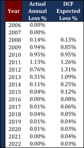
Using 2009 through 2022, let’s see how predictive the Wilary Winn DCF model is. Our results were highly predictive, with the exceptions of 2012, and especially 2013. The reason for the discrepancies is that we were hesitant to incorporate the very high rates of predicted increases in housing prices in 2013 into our modeling until the changes were realized3.
Next let’s look at how the expected losses would be recorded under CECL.
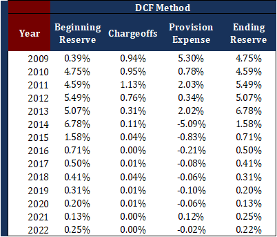
We can see the DCF model did a much better job predicting the losses to be incurred as of the 2009 year-end, resulting in a 4.75% reserve versus the WARM model’s prediction of 2.01%. As we alluded to earlier, we were too pessimistic regarding the losses at the end of 2013, and this combined with the aforementioned increase in average loan life required a significant increase in credit loss expense in 2013. When it became apparent that the increase in housing prices was real, the model released 5.09% of the portfolio balance. It released another significant amount in 2015, reflecting the improved credit outlook. In contrast, the WARM model released just 1.98% in 2014, followed by an additional required release of 1.49% in 2015.
The dollar effects on our hypothetical $500 million portfolio are shown below.
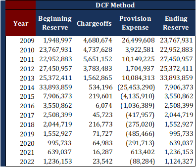
The table shows the DCF model largely worked as intended, capturing the beginning of the financial downturn in 2009 by increasing reserves and releasing three-quarters of the reserve in 2014 as credit conditions improved markedly.
The table below compares the provision expense and ending reserve using two different approaches. While the net provision expense totals approximately $21 million over the 14-year period, the WARM method grossly understates the required reserve in 2009 and does not release enough reserve in 2014.
Model Transparency
Under DCF, Wilary Winn uses the SIFMA cash flow standard because it is widely known, documented and accepted. We note that SIFMA standard discounted cash flow models are the analysis of choice for Wall Street. Hundreds of billions of asset-backed securities have been offered and sold based on their outcomes. Because of the size of the market, the financial mathematics involved are defined, documented, and well-known to financial industry professionals.
The loan attributes are transparent and relatively easily verified. The most important loan attributes for modeling are loan amount, interest rate, term, and loan-to-value. Loan amount, interest rate, term and original LTV can be traced to the loan accounting system.
Credit indicators are also transparent and relatively easily updated and verified. Current FICO scores and AVMs are readily available in the marketplace.
While not directly attributable to CECL, most of the credit indicators and collateral values would be considered Level 2 inputs in the fair value hierarchy. We note that the audit approach to fair value is robust and standard in the industry.
More importantly, the discounted cash flow model is prospective, not retrospective. The modeler is applying prepayment and default inputs to loan and credit attributes based on regional economic forecasts that are known at the time of modeling.
The portions of the model requiring the most review are the SIFMA standard calculations – is the financial math correct – and the regression analyses used to derive default and prepayment vectors.
Other Benefits
DCF modeling has other business advantages:
- DCF calculations underly the net economic value (“NEV”) for ALM models. Wilary Winn’s base scenario in our ALM offering is essentially the CECL reserve. More importantly, credit, interest rate, and liquidity risks can be and should be measured on an integrated basis.
- DCF models can be easily used for stress testing because they are prospective. Financial institutions can run multiple iterations of adverse macroeconomic circumstances and quantify the capital they have at risk.
- The same iterations can be run to set all-in loan pricing to ensure the interest rate is sufficient to cover expected credit losses under adverse scenarios. Because the model is run at the loan level, this analysis is relatively easily done.
- Strategic changes to lending can be easily communicated because the same primary variables used in the model – FICO and LTV – are the same ones used to make new loans.
Conclusion
In conclusion, the DCF model:
- Uses sophisticated financial mathematics;
- Can be used for multiple business purposes other than merely calculating the reserve;
- Is prospective and based on current loan and borrower credit attributes as well as current and forecasted macroeconomic conditions;
- Directly incorporates expected prepayments;
- Is transparent;
- Is highly predictive; and
- Does not require extensive qualitative and environmental adjustments.
Endnotes
- The sample is a multi-billion first lien portfolio of loans originated and retained by our credit union clients for which we were calculating fair value footnotes. ↩︎
- For the sake of simplicity and comparability, we are using the average life as determined by our DCF models. ↩︎
- Our sample portfolio is concentrated in California. Housing prices were expected to increase significantly in 2013. The actual increase per the FHFA HPI was 16 percent. Once we saw the predicted increases were real, we incorporated them into our model and our results were again highly predictive. Another key factor affecting 2013 was that the AVMs did not capture the recent increases in housing prices until the following year. ↩︎