Making the Business Case for the CECL Approach – Part I [White Paper]
Key Takeaway
We provide ALM and CECL solutions that help our clients measure, monitor, and mitigate balance sheet risk on an integrated basis. We consider credit, interest rate, and liquidity risk holistically. We charge a fee for our advice and do not rely on commissions, so we can remain objective. We simply want what is best for our client.
How Can We Help You?
Founded in 2003, Wilary Winn LLC and its sister company, Wilary Winn Risk Management LLC, provide independent, objective, fee-based advice to over 600 financial institutions located across the country. We provide services for CECL, ALM, Mergers & Acquisitions, Valuation of Loan Servicing and more.
Released December 2016
Introduction
This white paper is the first of a three-part series. We believe the implementation of CECL presents financial institutions with the opportunity to better integrate credit risk analysis across the organization. While it is imperative to understand expected life-of-loan credit losses in conjunction with the accounting requirements of CECL, this paper makes the business case that forecasted life-of-loan credit losses can be used to better manage an institution.
We believe the best managed institutions actively include credit risk management and lending personnel in their calculations. We further believe the best credit loss estimates are based on the same predominant credit indicators that the organization’s lenders use to make loans and that credit management uses to evaluate risk. Implementing the model across the organization using the same language utilized to make loans enables management to take direct action as needed. For example, it’s easier to have lending stop making loans below a specific FICO score and higher than a specific LTV, than it is to tell them stop making loans that are performing like the 2018 vintage.
We believe the best managed institutions measure, monitor, and manage credit, interest rate and liquidity risks on an integrated basis as part of their ongoing ALM process.
Attend any recent or upcoming financial institution conference and you will find considerable discussion and debate about the new accounting guidance related to the Current Expected Credit Loss Model (CECL) standard.
Effective in 2020 for SEC filers and 2021 for all financial institutions, the standard requires financial institutions to record lifetime expected credit loss estimates for loans, investments held to maturity, net investments in leases and off-balance sheet credit exposures. The new CECL standard is a departure from current practice because it removes the probability threshold that currently limits the amount that a financial institution can record in its ALLL. The financial impact of this change upon adoption will be a cumulative effect adjustment to retained earnings.
Wilary Winn LLC (“Wilary Winn”) believes the implementation of CECL presents financial institutions with the opportunity to better integrate credit risk analysis across the organization. Because the standard requires a prospective estimate, we believe the best managed institutions will actively include credit risk management and lending personnel in their calculations. In addition, we believe the best credit loss estimates will be based on the same predominant credit indicators that the organization’s lenders use to make loans and that credit management uses to evaluate risk. In other words, by prospectively considering how credit risk will change as economic conditions change based on quantitative indicators, instead of performing a lookback analysis to calculate a reserve required for accounting, we believe a financial institution can better manage risk.
While it is imperative to understand lifetime credit losses in conjunction with the accounting requirements of CECL, this paper makes the business case for an organization to forecast lifetime credit losses by demonstrating the numerous advantages of adopting this approach within the asset liability management framework. Said another way, financial institutions should forecast lifetime credit losses for business advantages even absent the CECL requirements.
While determining lifetime credit loss exposure on loan and investment portfolios is new to some in the industry and the requirement is being met with skepticism by many, Wilary Winn notes that life of loan credit loss estimates are required now under GAAP for many items including calculations of:
- Other-than-temporary impairment of debt securities
- Troubled debt restructurings
- Accretable and non-accretable income estimates
- Fair value estimates for loans and investments acquired
Indeed, we have been providing lifetime credit loss estimates to our clients for these items since 2009. In addition, our economic value of equity (EVE) calculations for our Asset Liability Management (ALM) product offering have included lifetime credit loss estimates based on credit attributes since we began offering the service. Were we clairvoyant in forecasting the arrival of CECL and looking for advanced preparation – not at all. We included lifetime credit loss estimates as part of our ALM process because we strongly believe that interest rate risk, credit risk and liquidity risk should be examined on an integrated basis. Moreover, because failure to manage credit risk has been the primary culprit for most banking crises historically, one can reasonably argue that credit risk is the most critical of the three. Based on the importance of managing credit exposure, we found it completely unacceptable to merely utilize the ALLL reserve currently required under GAAP for ALM modeling purposes. We provide lifetime credit loss calculations as part of our ALM service offering in order to provide our clients with feedback on their credit exposure so that they can ultimately optimize their balance sheets. Incorporating credit loss modeling within base case and stressed economic environments, combined with multiple interest scenarios, allows an organization to gain better understanding of the balance between return and capital at risk in pursuit of returns – thus allowing it to proactively manage its balance sheet.
Even if the CECL standard were to be withdrawn, Wilary Winn would continue to incorporate credit loss modeling as part of ALM to help our clients achieve best practices with:
- Loss exposure analysis
- Capital stress testing
- Business strategy evaluation
- Concentration risk management
- Risk based pricing and real return
This white paper focuses on loss exposure analysis, capital stress testing and evaluating a business strategy based on an increase in leverage. Look for our upcoming white papers, which describe how to use lifetime credit loss estimates to develop:
- Quantitative concentration limits
- Loan pricing based on real expected returns
Wilary Winn believes that the best way to evaluate a loan portfolio’s risk/return profile and understand the related trade-offs is to calculate lifetime expected credit losses under multiple economic environments using discounted cash flow analyses. We will begin with the basics.
The Building Blocks
Let’s begin by describing the primary model input assumption we need to calculate lifetime credit loss estimates. For a given loan or loan cohort, we must develop model input estimates for:
- Voluntary prepayment – conditional repayment rate (“CRR”)
- Involuntary prepayment – conditional default rate (“CDR”)
- Loss severity if a default occurs
To best apply these assumptions, we first stratify the portfolio by loan attributes. For example, we separate first lien residential real estate loans from junior lien. We further divide the first liens into fixed and variable, and junior liens between closed and open-ended. For auto loans, we separate new from used, and further segment by direct and indirect. We do this because our modeling experience has shown that these loan types perform differently even with similar credit indicators.
We then segment the loan categories by predictive credit indicators. For residential real estate loans, we use FICO and combined loan to value. For other consumer loans, we rely primarily on FICO. For commercial loans we typically apply the credit assumptions by risk rating, debt service coverage and NAICS code.
Our next step in the process is to determine input assumptions for voluntary repayment, involuntary repayment, and loss severity to apply to the stratifications and segments. We do this based on our analysis of the historical performance of billions of dollars of loans across the most recent ten-year business cycle. We have performed multiple regression analyses in order to develop the detailed CRR, CDR and severity loan assumptions to be applied to a given loan cohort. We continue to benchmark our assumptions to our client’s actual performance and other industry sources. We regularly back-test our results and continue to implement modeling improvements. Our experience forecasting lifetime credit losses for billions of dollars of loans to date has led us to believe that accurate forecasts require analyses of large pools of data across a full business cycle combined with the rigorous processes we have and continue to undertake.
In addition to analyzing lifetime credit losses in a base case economic environment, we believe our clients should consider the sizeable additional lifetime credit losses that could occur if adverse economic conditions were to arise. Conditional default rates increase exponentially in adverse economic environments, particularly for the low credit groups. Even if the risk/return trade-off makes financial sense in the current economic environment, we believe financial institutions should include realistic worst case scenarios in determining the amount of capital it should put at risk in pursuit of returns. Risks that threaten the long term financial health of the institution should never be undertaken. Because economic conditions change, Wilary Winn’s loss forecasts are based on multiple economic environments.
This leads to a question – which economic variables have the most influence on loan performance metrics. We have found that certain economic variables are highly correlated to forecasted loan performance. For most loan types, the change in the unemployment rate is the most highly correlated to loan performance. To best illustrate the relationship between unemployment and loan delinquency and demonstrate our rationale for our multi-economic environment approach, the following graph shows the unemployment rate and 1st mortgage delinquency rate over the most recent business cycle for the United States, California and Los Angeles.
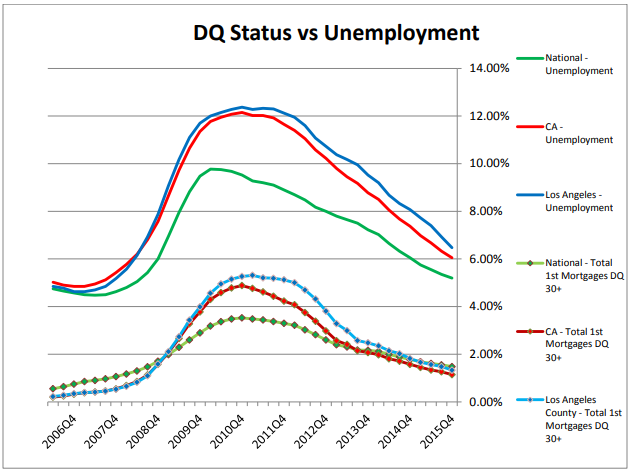
In analyzing unemployment rates and 1st mortgage 30+ day delinquency data (delinquencies are leading indicators of default) through the Financial Crisis, we note extremely strong correlation coefficients of 93.4%, 97.0% and 94.5% to the U.S., California and Los Angeles markets, respectively. Wilary Winn has calculated 1st mortgage 30+ delinquencies correlation coefficients to numerous macroeconomic variables and unemployment rate reflects the strongest correlation by far. As a result, our lifetime credit loss stress tests are based on economic environments with high unemployment rates. Our default rate stress factors are based on further analysis of the past relationship between unemployment and delinquencies. Based on this analysis, we can estimate default rates for the levels of unemployment rates our clients want to assume when developing economic stress analyses of expected lifetime credit losses.
Estimating Lifetime Credit Losses
With our basic methodology developed, we are now ready to examine and interpret lifetime credit loss results. The following table shows an example of aggregate credit loss calculations by loan type for a hypothetical one-billion-dollar loan portfolio under multiple economic environments. We generated our estimates of lifetime losses by applying CRR, CDR and loss severity model input assumptions at the loan cohort level. As a reminder, the delinquent and low FICO loan groups incur the highest rates of default. To further our example, we have also included agricultural loans. We developed our stress test for the agricultural loans based upon an economic environment of low commodity prices in addition to a high unemployment rate. We did this to show the importance of selecting the appropriate credit indicators to use when developing model input assumptions because defaults on agricultural loans correlate strongly with commodity prices but poorly with the unemployment rate.
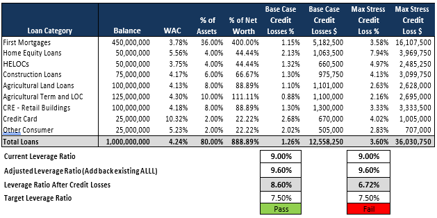
As the previous table shows, based on the current economic environment (unemployment at 4.5%), we estimate that lifetime credit losses will be approximately $12.6 million or 1.26% of unpaid principal balance. Under a stressed economic environment, defined as the unemployment rate being elevated to and remaining at 10.2% (the peak national unemployment rate during the Financial Crisis) along with low commodity prices, we project lifetime credit losses to increase to $36.0 million or 3.60% of unpaid principal balance.
We believe the knowledge gained from the credit stress analyses can be used for capital stress testing and concentration risk analyses – how much capital should a financial institution put at risk in pursuit of return and how to ensure it does not inadvertently put too much capital at risk by not fully considering concentration risks.
Extremely well-capitalized institutions can afford to undertake greater amounts of risk in pursuit of returns, while those with less capital can undertake relatively less risk. While financial institutions have varying degrees of risk tolerance, let’s assume that the organization in our example wants to maintain capital in excess of 7.50% in both the base case and in an adverse economic environment of sustained high unemployment and low commodity prices. The previous table also shows the effects the estimated lifetime credit losses would have on its capital level under a base case and maximum stress scenario.
Our example financial institution has a net worth of 9.00% on an overall balance sheet of $1.25 billion and an ALLL reserve under the current accounting standards of 0.60%. As demonstrated by the previous table, the example financial institution thus has an adjusted net worth of 9.60% (ALLL added back to capital) before including lifetime credit losses under the CECL standard. Lifetime credit losses are then deducted from the adjusted leverage ratio. In the base case, where the unemployment rate remains at 4.5%, net worth after lifetime credit losses is 8.60% substantially above the 7.50% internal threshold. However, the higher forecasted losses resulting from the stressed economy with sustained 10.2% unemployment and low commodity prices results in a net worth ratio after lifetime credit losses of 6.72%, well below the 7.50% internal threshold. Based on this organization’s risk tolerance, it must adjust its balance sheet in order to better withstand adverse economic conditions. Ideally, the adjustments made will allow the organization to earn a similar return and decrease risk. In the sections that follow we describe how to evaluate changes in the loan portfolio mix and optimize the risk/return relationship based on an organization’s risk tolerance.
Change in Loan Mix
Our goal is to reduce our example financial institution’s credit risk exposure in the adverse economic scenario (high unemployment and low commodity prices) in order to maintain 7.50% capital. To accomplish this goal, the organization will change its loan mix. To do this, it will first develop a more granular understanding of its potential credit losses. The following table reflects a more detailed look at our example institution’s credit losses. The loan categories are further stratified by credit grade: low risk, medium risk, and high risk. By further examining the credit grade stratifications, we learn that this particular example financial institution experiences significant financial detriments from its higher risk loans in the stress scenario. In particular, the loss rate from high-risk residential real estate loans triples in the stress scenario. The results suggest that the more ideal balance sheet for this organization would have less exposure to high-risk lending in general, and especially to less overall high-risk exposure to residential real estate. As illustrated in the following table, with no net changes in the loan portfolio total, the organization could significantly reduce its credit loss exposure in both the base case and economically stressed credit environments by reducing its reliance on the high-risk credit categories. By reducing its first mortgage loan exposure, increasing its exposure to agricultural sector, and improving the credit profile, it can reduce its base case loss rate from 1.26% to .72% and, more importantly, to 2.10% in the stress scenario from 3.60%. This allows it to remain at the targeted minimum capital threshold of 7.50%, thus assuring the institution maintains sufficient amounts of capital in the face of economic adversity.
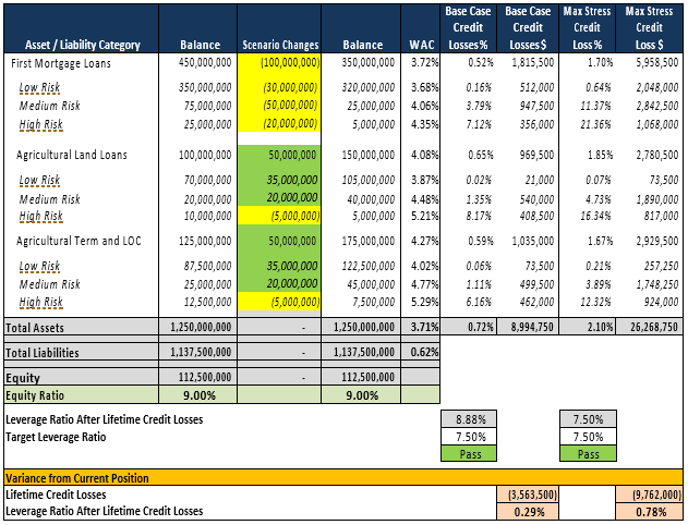
Of course, we realize that the instantaneous change we made in the model cannot, in reality, be instantly duplicated. That said, the organization now has a path to reducing its credit risk profile over time because the lifetime credit loss analyses clearly demonstrated the risk/return profile of the high-risk loans was unfavorable to the financial institution.
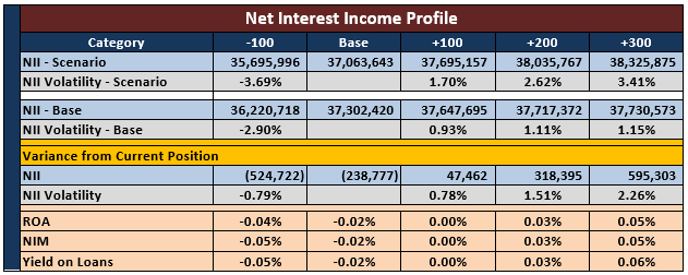
Now that we have analyzed lifetime credit losses and capital at risk, we will next consider the effect the changes in loan mix will have on income and interest rate risk and return by analyzing net interest income and economic value of equity under multiple interest rate environments. As reflected in the following table, net interest income decreased slightly in the base case but increased in rising rate scenarios mainly due to the lower exposure to long term, fixed rate residential real estate loans. For the substantial capital at risk benefit, the organization receives slightly less net interest income in the base case scenario.
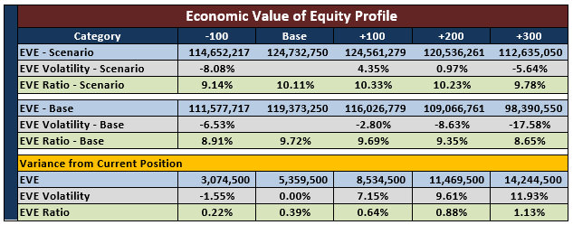
In examining long term interest rate risk exposure changes of our loan reallocation strategy as measured with economic value of equity analysis, the change in loan mix results in slightly less overall interest rate risk exposure. This is the expected result with the reduction of long-term, fixed rate residential lending. Following is a table that shows that the EVE ratio has improved and there is less volatility in the rising rate scenarios.
Up to this point, we have analyzed credit risk and interest rate risk separately. The following table shows an integrated view of credit risk and interest rate risk for the change in loan mix strategy. The goal of this table is to provide a summary of relevant credit and interest rate risk information to facilitate a comprehensive and integrated evaluation of the business strategy. The table highlights the effects of the change in loan mix strategy:
- Reduced credit exposure in the base case max economic stress scenarios
- Decreased interest rate risk due to the reduction of fixed rate residential mortgages
- Minimum impact to net interest income
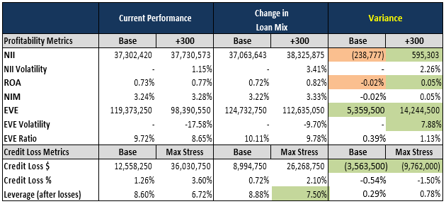
Based on our integrated analysis, adjusting the loan mix to focus on higher credit loans and less residential mortgages makes sense given the example financial institution’s risk tolerance because it can generate similar net interest income with less overall credit exposure. Even in the event of an adverse change to the economy, the organization’s capital level will remain strong, and the organization will continue to thrive.
Adding Leverage
Let’s now examine and evaluate another type of business strategy. This time we will focus on increasing returns. For our analysis, we will begin with our example financial institution’s beginning balance sheet before we changed the loan mix. We now assume that the example financial institution has a higher risk tolerance. We change the credit loss and capital level test thresholds to maintain capital in excess of 7.50% in the base case economic scenario (the same as before) but to 6.00% in the maximum stress economic scenario. To increase the overall profitability of the financial institution, it implements a leverage strategy where assets and liabilities each increase by $100 million. The specific balance sheet adjustments are shown in the following table. With the leverage strategy, the nominal amount of equity remains at $112.5 million but the equity percentage decreases from 9.00% to 8.33% given the $100 million increase in total assets. The purpose of this exercise is to provide another realistic example on how examining credit risk and interest rate risk on an integrated basis can lead to increased optimization of a financial institution’s risk/return profile.
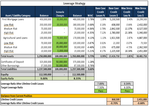
The $100 million increase in loans generates additional lifetime credit losses. Lifetime credit losses increase $869k in the base case economic scenario and $2.45 million in the maximum economic stress scenario. While additional credit losses are incurred with the leverage strategy, the losses are still within the organization’s risk tolerance as the equity percentage is above the 7.50% tolerance in the base case and above 6.00% tolerance in the maximum economic stress scenario. These additional losses are just one component of the risk/return tradeoff analysis. The next steps are to evaluate profitability and interest rate risk exposure.
The net interest income benefit to the organization of the leverage strategy is substantial. As reflected in the following table, the effect of adding $100 million in assets and liabilities increases 12-month net interest income by $2.9 million in the base case scenario. The net interest income benefit is reduced slightly with instantaneous and parallel shifts of rising market interest rates. However, this strategy is advantageous to the organization as return on assets increases in all scenarios modeled.
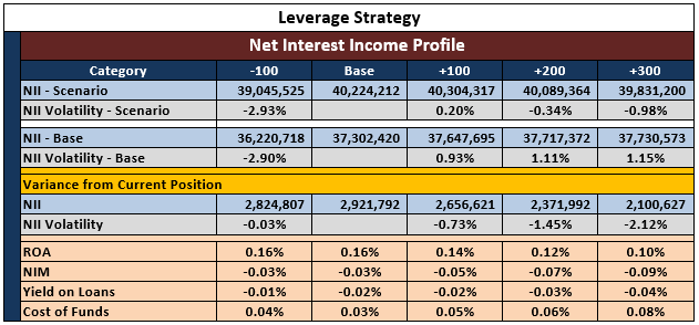
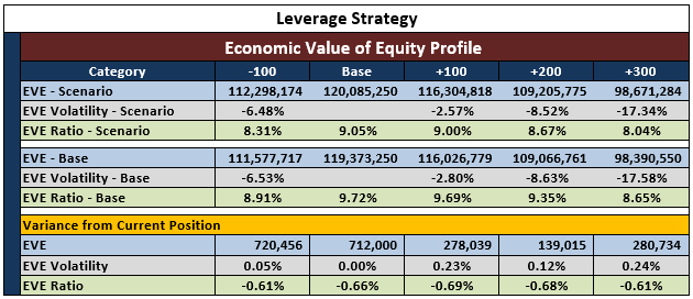
In our analysis of long-term interest rate risk as measured with economic value of equity analysis, the leverage strategy results in a much lower EVE ratio in all modeled interest rate risk scenarios. Volatility is similar when we compare the leverage strategy to the starting balance sheet position. The following table reflects the long-term interest rate risk profile of the leverage strategy in comparison to the beginning balance sheet.
In the following table we summarize our integrated analysis of interest rate risk and credit risk for the leverage strategy. It shows the opportunities of the potential strategy – greater net interest income and elevated return on assets. It also shows the risks – increased lifetime credit losses in the base case and stressed economic environments. Additionally, this table shows that the increased credit risk is still within the overall risk tolerance of the organization as capital exceeds 7.50% in the base case and 6.00% in the maximum stress environment.
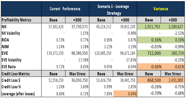
Wilary Winn believes that this table offers a comprehensive summary of the effects of undertaking the proposed strategy and can be used by financial institution managers to make more informed and better decisions as they evaluate alternatives when planning. While it is impossible to remove all risk from a financial institution’s balance sheet, understanding and proactively managing the risk/return tradeoff can help ensure long-term business success.
Conclusion
While financial institutions must begin to prepare now in order to become compliant with the required CECL provisions by 2021, Wilary Winn believes there are multiple business rewards to incorporating lifetime credit losses within the framework of the asset liability management process now.
We believe that fully incorporating lenders and credit risk managers into the estimation process using the credit indicators with which they are familiar can lead to better communication across the organization, and thus to more effective decision making.
This paper demonstrated the advantages of examining the risks and opportunities a financial institution faces on an integrated basis. We believe an understanding of the losses an institution could incur under multiple macroeconomic conditions can lead to better capital allocation decisions, improved profitability, and an organization better able to withstand economic downturns.